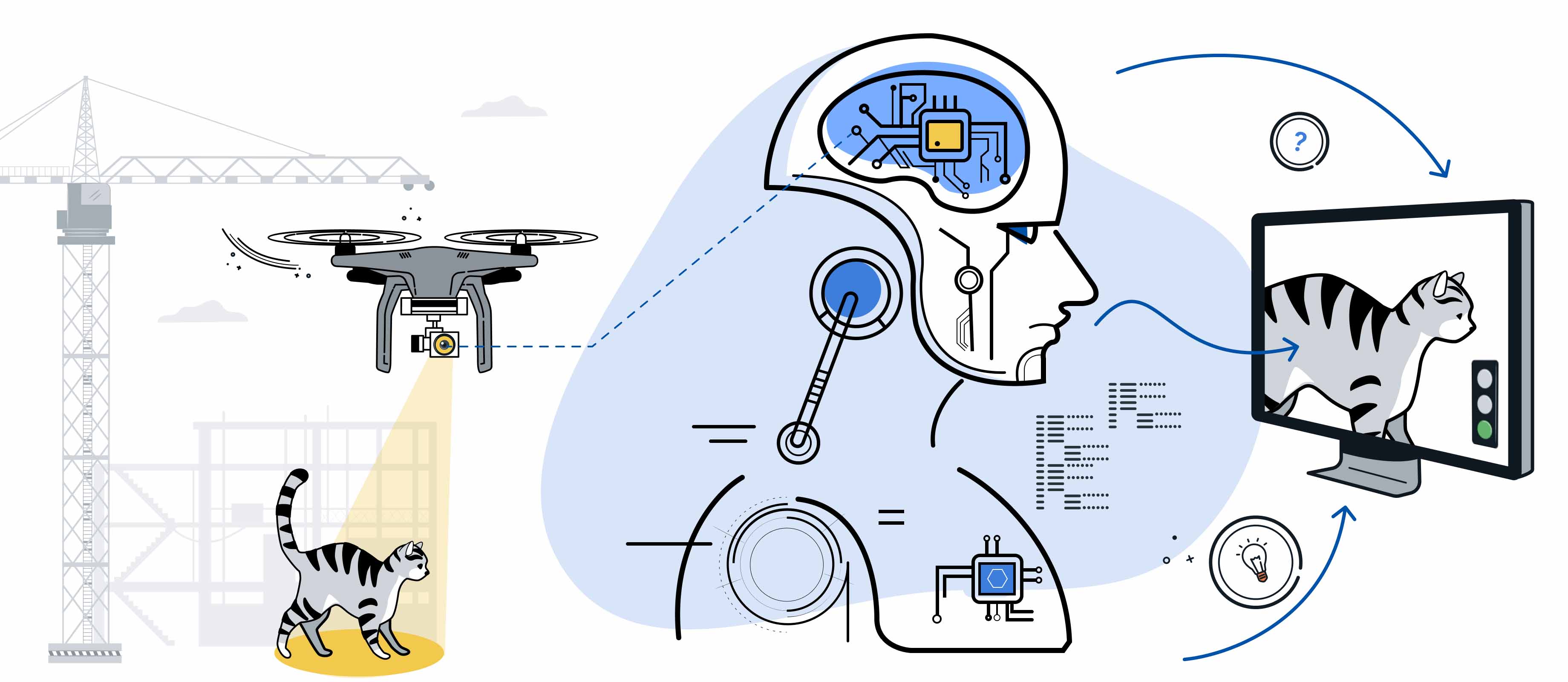
It originated in antiquity and its ideas continue to drive revolutionary inventions to this day. What for a long time was only found in myths and fictional works has now had a permanent place at the forefront of science for several decades. In dystopian world scenarios, it seizes complete control of the planet and yet it is able to optimise our lives in almost every area: Artificial intelligence.
In our current blog post, our Xperts examine a particular branch of this sub-discipline within computer science: Machine learning. This sub-discipline deals with the learning ability of machines - the artificial production of knowledge. Using a compact example with Python, our Xperts show how a model can recognise numbers with the help of machine learning algorithms. To begin with, however, we would like to clarify a few terms and concepts for a better understanding.
Artificial intelligence
Artificial intelligence refers to any process that uses a computer algorithm to train a model. The word artificial first establishes that it is something that does not occur in nature. Intelligence is defined here as the ability to direct actions towards goal attainment - tasks in which machines are supposed to work in a human-like manner.
The trained model can be applied to environmental perception and decision-making. However, the model requires input data in order to be useful in this role. Artificial intelligence is therefore dependent on a realistic representation of, for example, sensor data or other input variables. The method for training these models is called machine learning.
Machine Learning
With the help of machine learning algorithms, machines are able to learn from data and recognise patterns. On this basis, they can take human-like actions such as making predictions or decisions.
To train a model, machine learning uses predefined features that are taken into account by the model. Humans have a significant influence in the selection of these features through multi-faceted pre-processing in the creation process. This radius of action facilitates feature extraction on the finished model.
Feature extraction is a method in machine learning that can be used to determine the most meaningful input variables. For example, in image classification tasks, the output could be which pixels will most likely be assigned to which object.
If you go one step further or deeper in machine learning, you enter the realm of deep learning. Unlike machine learning, this sub-area concentrates on the hidden layers of a model. To train the model, the features are no longer defined by humans. Since several steps are omitted before training, control over the result is lower than with traditional machine learning methods. The first training steps - the warm-up - are a random mixing of the features. With the help of the hidden layers, the model then decides during the training process which features are the most relevant.
Since this special form of artificial intelligence requires enormous amounts of training data and computing power, and therefore also incurs a high cost, deep learning is not suitable for broad applications. Whereas with machine learning everything could still be calculated by hand, this is no longer possible with deep learning. The complexity of the calculations is no longer comprehensible for humans in individual cases.
Regardless of whether it is machine learning or deep learning, the core of both is formed by so-called artificial neural networks.
Artificial neural networks
The structure and function of artificial neural networks are modelled on the human brain. They are ideally suited for automating tasks in order to recognise patterns or correlations in large amounts of data. The foundation of every artificial neural network is formed by many interconnected computing units - the artificial neurons.
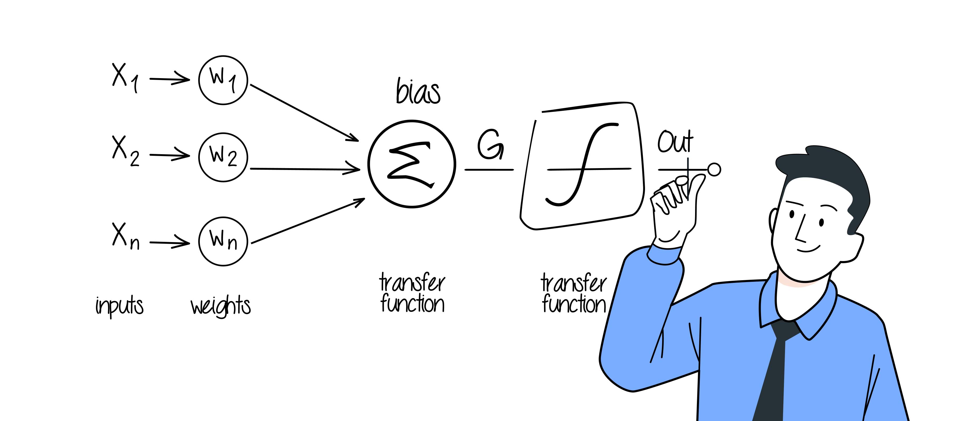
An artificial neuron is composed of several inputs, each of which receives a signal, and an output, which sends out the signal. Each input value is assigned a so-called weighting, which regulates the contribution of this input to the total output of the neuron. The weighted input values are then added together and transmitted to the activation function for output.
In an artificial neural network, each of these artificial neurons is connected to each other and, in deep learning, even across several layers.
Performance metrics
An important tool to determine the performance of machine learning models are performance metrics. These are evaluation metrics and the suitability of each metric is dependent on the use case. In the following, we would now like to give a brief overview of the most common of these operations.
| Value | Symobl or formula | Definition |
|---|---|---|
| True Positive | tp | Positive data classified positive |
| True Negative | tn | Negative data classified negative |
| False Positive | fp | Negative data classified positive |
| False Negative | fn | Positive data classified negative |
Accuracy: Accuracy determines how often the model predicts correctly. It is calculated by dividing the number of correct predictions by the total number of predictions.
Precision: Precision determines how often the model makes correct positive predictions. It is calculated by dividing the number of correct positive predictions by the total number of positive predictions.
Recall (Sensitivity): Recall is used to determine how often the model has identified all actual positive cases. It is calculated by dividing the number of correctly identified positive cases by the total number of actual positive cases.
F1 score: The F1 score is the harmonic mean of precision and recall. This makes the F1 score less susceptible to misleading accuracy values and has established it as the standard for accuracy assessment.
Using these metrics, it is easy to see whether a system is biased too strongly on one side. In order to achieve the desired result, the parameters can be adjusted if necessary, for example by adding a new bias at the end.
Hardware requirements
In principle, almost all common PCs or laptops are sufficient to run machine learning. Even for complex applications, the computing power of these devices is sufficient. For example, single-board computers such as the Raspberry Pi can also be used to get started with machine learning. In deep learning, however, the hardware requirements are considerably more demanding. Due to the artificial neural networks with several layers and the complex calculations, entire computer centres are sometimes required to carry them out. The larger and more complex the model, the faster the requirements for the necessary hardware increase.
Application
Now that the basic terms and concepts have been clarified, we would like to go into our practical example with Python. For this, we will work on pixel-based number recognition with a logistic regression. This is a mathematical function for mapping the model to be trained.
Jupyter Notebooks (.ipynb), for example, is ideal for learning, as the code can be broken down into individually executable blocks. Jupyter is available as a standalone version, but also as a plug-in for popular code editors.
First of all, the required libraries must be imported into Python.
import numpy as np
import sklearn
import matplotlib.pyplot as plt
import pandas as pd
%matplotlib inline
The MNIST dataset from the National Institute of Standards and Technology is freely available and contains a variety of training and test data. This can be downloaded and imported in Python with the following code:
from six.moves import urllib
from scipy.io import loadmat
mnist_url = "https://github.com/amplab/datascience-sp14/raw/master/lab7/mldata/mnist-original.mat"
mnist_path = "./mnist-original2.mat"
response = urllib.request.urlopen(mnist_url)
with open(mnist_path, "wb") as f:
    content = response.read()
    f.write(content)
mnist_raw = loadmat(mnist_path)
mnist = {
    "data": mnist_raw["data"].T,
    "target": mnist_raw["label"][0],
    "COL_NAMES": ["label", "data"],
    "DESCR": "mldata.org dataset: mnist-original",
}
The now declared "mnist" variable must still be divided into training and test data. For our example we use 60,000 training data and 10,000 test data.
from sklearn.model_selection import train_test_split
X_train, X_test, y_train, y_test = train_test_split(mnist['data'], mnist['target'],train_size=6/7, test_size=1/7,random_state=101)
Data exploration and pre-processing
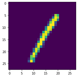
The data contained in the MNIST dataset are images with a resolution of 28x28 pixels.
With the command plt.imshow(X_test[0].reshape(28,28)) the first image in the test data set can be displayed.
To start training the machine learning model, it must first be imported with from sklearn.linear_model import LogisticRegression and defined as model=LogisticRegression().
The frequency with which the model should iterate through the training data set is defined with model.max_iter=4. The choice of iterations is of great importance in machine learning. If a model is under-trained, it may not be able to generalise the "features" to be recognised. An overtrained model, on the other hand, may be very accurate when tested against the training dataset, but would perform significantly worse against new test datasets.
Finally, the training can be started with model.fit(X=X_train, y=y_train).
Due to the low number of iterations, training data and pixels to be processed per image, this model is completely trained within a few seconds. This is also due to the computing power of today's hardware.
To be able to determine the accuracy of the model, the accuracy values are needed. These can be calculated by sklearn with the following code:
from sklearn.metrics import classification_report, confusion_matrix
y_train_pred_first = model.predict(X_train)
y_pred = model.predict(X_test)
plt.matshow(confusion_matrix(y_test, y_pred))

y_train_pred = model.predict(X_train)
y_test_pred = model.predict(X_test)
print(classification_report(y_test, y_pred))
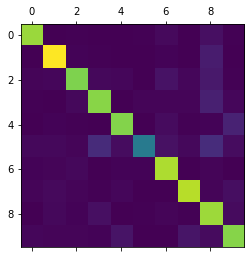
The resulting confusion matrix describes which numbers the model recognises correctly.
In this diagram, the number 5 is not very pronounced and there are clear deviations in the numbers 3 and 8. This means that 5 is particularly poorly recognised as such by the model and is often misrecognised as 3 or 8.
The trained model
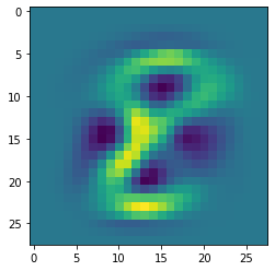
With the command plt.imshow(model.coef_[8].reshape(28,28)) the coefficients of a model (here the number 8) can be visualised. The bright, yellow areas represent those pixels that the model clearly associates with the number 8. However, if a pixel is in a dark blue area, this speaks against a classification as 8.
For each number to be recognised, a probability for the possible numbers 0 to 9 is output at the end of the processing chain at the output neuron. The number with the highest probability is used as the recognised number at the end.
!
Excursus data preprocessing
In machine learning, pre-processing of data is essential to achieve better results. The MNIST dataset has already been cleaned of many sources of error.
Possible pre-processing in the case of number recognition includes reducing brightness information, edge enhancement or realigning the numbers to the centre of the image. It may be worthwhile to try these methods and then compare the accuracy values. For this, only the values of X_train and X_test have to be replaced.
Information reduction
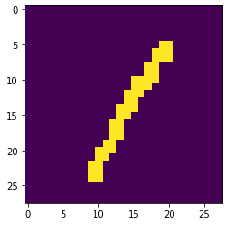
In the case of the MNIST data set, brightness values from 0 to 255 are available (8 bits). The brightness values can be determined using X_train.min() and X_train.max(). This information can be reduced to 1 bit, for example, by determining a threshold value below which all values are defined as 0 and above which all values are defined as 1.
from sklearn.preprocessing import minmax_scale, binarize
X_train_binarized = minmax_scale(X_train)
X_test_binarized = binarize(X_test, threshold=96)
With this method, the input data for the machine learning model was reduced by a factor of 128. However, the accuracy decreases by 1 % in the F1 score due to this pre-processing. The example clearly shows that in machine learning, models can often be downscaled for weaker hardware or limited data transmission paths without having to accept a large loss in accuracy.
Edge detection
Another method of data pre-processing is the creation of images using edge detection. Image manipulations can be carried out with the Python Image Library PIL. After this has been imported, the pixels of the training data must be read in as images. Then edge detection can be applied to them. To be able to use the images later as training data, they have to be written again as individual pixels into an array. This process is repeated with the test data set. The resulting array has three dimensions, but our model can be trained with a maximum of two dimensions. The dimensions can be reduced with np.concatenate.
from PIL import Image, ImageFilter
X_train_pil = [Image.fromarray(x.reshape(28, 28)) for x in X_train]
X_train_pil_edges = [x.filter(ImageFilter.FIND_EDGES) for x in X_train_pil]
X_train_edges = np.array([np.array(x).reshape(-1, 784) for x in X_train_pil_edges])
X_test_pil = [Image.fromarray(x.reshape(28, 28)) for x in X_test]
X_test_pil_edges = [x.filter(ImageFilter.FIND_EDGES) for x in X_test_pil]
X_test_edges = np.array([np.array(x).reshape(-1, 784) for x in X_test_pil_edges])
X_data_train = np.concatenate([X_train, X_train_edges[:, 0, :]], axis=1)
X_data_test = np.concatenate([X_test, X_test_edges[:, 0, :]], axis=1)
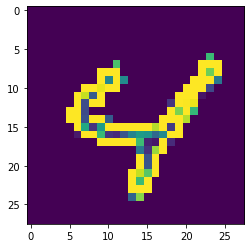
This data pre-processing also unfortunately does not bring any gain in accuracy in the F1 score with an accuracy loss of 2 %. The images in the MNIST dataset are already well pre-processed for further processing. However, our small experiment shows that numerous options exist for feeding data to a machine learning model.
How do we work?
Machine learning can be used in many different ways. It makes a valuable contribution to the realisation of predictive maintenance applications in our projects. For example, based on an artificial neural network, we have developed an application that automatically recognises devices that need to be serviced.
In the future, the industries in which machine learning will be an important factor will expand further, not least due to continuously improving hardware performance. Due to its lightweight nature, machine learning will also endure alongside deep learning in driving technological change for a long time to come.
Data Science
Learn more about our services